[머신러닝개론] 3. First-Order Optimization

 

1. First-order optimization methods

- 기초적인 최적화 알고리즘(optimization algorithms)으로, 1차 미분이나 함수의 gradient를 사용한다.

- keyword: ① the first-order optimality condition ② hyperplanes ③ the first-order Taylor series approximation ④ gradient descent algorithm

---

1) The first-order optimality condition

1-1) The first-order optimality condition

- the first-order optimality condition: the derivative or gradient of a function = 0

: the line or hyperplane tangent to a function has zero slope.

: 하지만, 반드시 그런 것은 아님. 변곡점(saddle point), 최솟값, 최댓값, 값 자체가 0 등 경우는 다양함.

- a potential minimum: 미분값 = 0인 지점

: N-dim input,

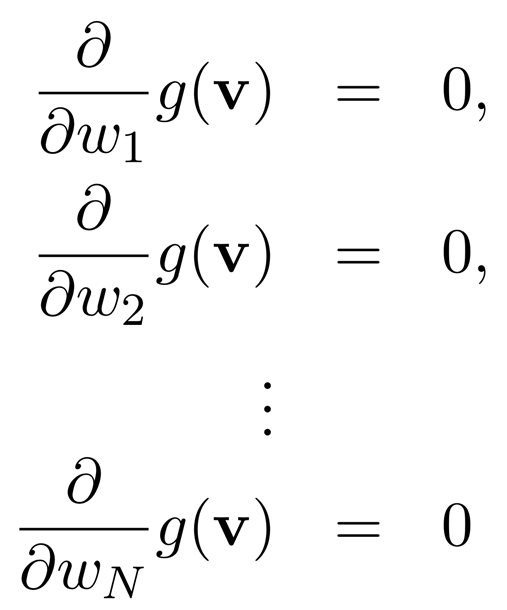
간단히 적으면,

gradient

---

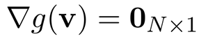
1-2) Coordinate descent and the first-order optimality condtion

- zero-order optimization에서 본 것처럼, 순차적으로 한 변수만 남긴 채 다른 모든 변수는 상수로 고정하고 변수 하나씩 미분해주는 것이다. (한마디로, 편미분)

---

2) The Geometry of First-Order Taylor Series

- Hyperplane(초평면)

: ① 2차원의 Hyperplane은 직선 (ax + by + c = 0) ② 3차원의 Hyperplane은 평면- (ax + by + cz + d = 0) ③ 4차원의 Hyperplane은 3차원 (aw + bx + cy + dz = 0)

: 공간을 분할할 수 있다.

: 갑자기 초평면 이야기를 왜 꺼내냐면, 이를 이용해 하강법 d를 구할 것이기 때문이다.

2-1) N-dim hyperplane

$h(w_1,w_2,...,w_n)=a+b_1w_1+b_2w_2+...+b_nw_n$h(w1​,w2​,...,wn​)=a+b1​w1​+b2​w2​+...+bn​wn​​

$h\left(\overrightarrow{w}\right)=a+\overrightarrow{b}^T\overrightarrow{w}$h( w)=a+ bT w​

$b^T=[b_1,b_2,...,b_n]$bT=[b1​,b2​,...,bn​]​

$w=\left[w_1,w_2,...,w_n\right]^T$w=[w1​,w2​,...,wn​]T​

2-2) Steepest ascent and descent directions

- To find the direction of steepest ascent at w^0.

- h: hyperplane을 의미

(최솟값을 찾는다면서 max라고 쓴 이유는, 최대로 변하는 방향의 반대방향으로 가주면 최소가 되는 방향이기 때문이다.)

$\max _d^{ }\ h\left(w^0+d\right)\ for\ all\ unit-length\ vectors\ d.$maxd h(w0+d) for all unit−length vectors d.​

2-3) The gradient and the direction of steepest ascent/descent

- d를 변화시키며 최솟값을 찾는 것이기 때문에 d가 없는 모든 값은 상수로 취급하고 무시한다.

내적 (b^T)(d)를 최댓값으로 만들려면 두 벡터가 같은 방향을 바라보면 된다.

$\max _d^{ }\ h\left(w^0+d\right)\ =\ \max _d^{ }\ a+b^T\left(w^0+d\right)\ =\ \max _d^{ }\ \left(b^Td\right)$maxd h(w0+d) = maxd a+bT(w0+d) = maxd (bTd)​

d = b/||b|| : the steepest ascent

d = -b/||b| : the steepest descent

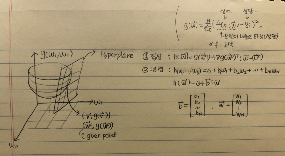
- w^0: given point (일정한 값들의 모임이기 때문에 상수)(초기지점. 예를 들어 (w_0, w_1) = (1, 2)에서 시작할 때 그 위치), a 또한 상수이다.

 

2-4) 중간 정리

(given point를 (v, g(v))와 (w^0, g(w^0)) 두 가지 표기법으로 적고 있음)

The Geometry of First-Order Taylor Series의 내용을 정리해보도록 하겠습니다.

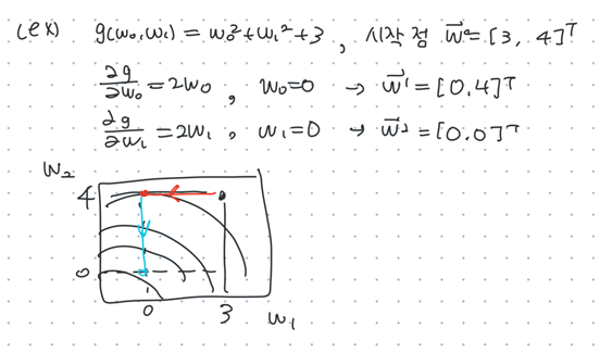
loss function(g(w))를 줄이기 위해 given point(v, g(v))에서 제일 급격하게 g(w)가 감소하는 부분으로 내려가고자 합니다. 이는 해당 점(v, g(v))에서 접평면(Tangent plane, hyperplane)을 구한 후 max(b^Td)를 만드는 d를 얻으면 된다는 걸 배우게 되었습니다.

the steepest descent(d)는 hyperplane의 b를 이용해 구할 수 있습니다.

그렇다면, b는 어떻게 구할까요? tailor approximaition을 통해 얻을 수 있습니다. 대학교 미분적분학2에선 선형근사(linear approximation)이라는 이름으로도 불립니다.

 

2-5) tailor approximation

(정확히 말하면 hyperplane 표기법②라고 하기 애매하지만, hyperplane=접평면인 상황이므로 이렇게 표기)

given point에서 접평면은 tailor approximation을 통해 얻을 수 있다. 이는 위에서 언급한 hyperplane과 같은 것이다.

$y=y_0+\frac{dy}{dx}_{x=x_0}\left(x-x_0\right)$y=y0​+dydx​x=x0​​(x−x0​)​

$h\left(w\right)=g\left(w^0\right)+▽g\left(w^0\right)^T\left(w-w^0\right)$h(w)=g(w0)+▽g(w0)T(w−w0)​

이는 tangent plane approximation입니다. 2변수함수로 예시를 들어보자면 아래 식과 똑같은 의미입니다.

$z-z_0=f_x\left(x_0,\ y_0\right)\left(x-x_0\right)+f_y\left(x_0,\ y_0\right)\left(y-y_0\right)$z−z0​=fx​(x0​, y0​)(x−x0​)+fy​(x0​, y0​)(y−y0​)​

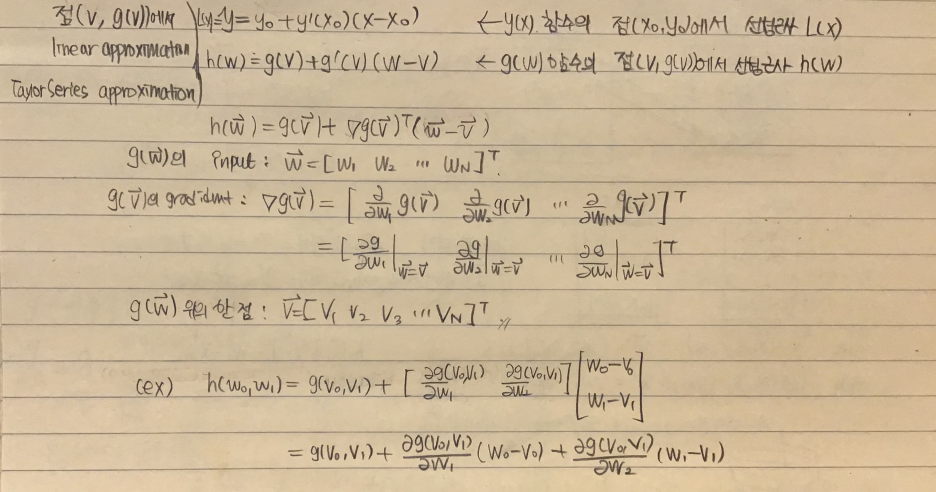
(x_0, y_0, z_0) 점 위에서 z = f(x, y)에 관한 접평면이죠. 이를 좀 더 깔끔히 정리했다고 보시면 됩니다!

 

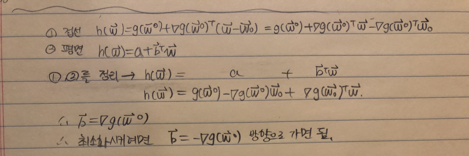
2-6) the steepest descent(d)

(2-1)N-dim Hyperplane 과 (2-5)tailor apporoximation은 같은 평면을 나타내므로 이를 정리해준다.

3) The gradient descent algorithm

$w^k=w^{k-1}+\alpha d^k$wk=wk−1+αdk​

$d^k=-▽g\left(w^{k-1}\right)$dk=−▽g(wk−1)​

(1) Steplength ① α = 10^-k ② α = 1/k

α에 따라 Oscillation in the cost function history plot이 일어나기도 한다.

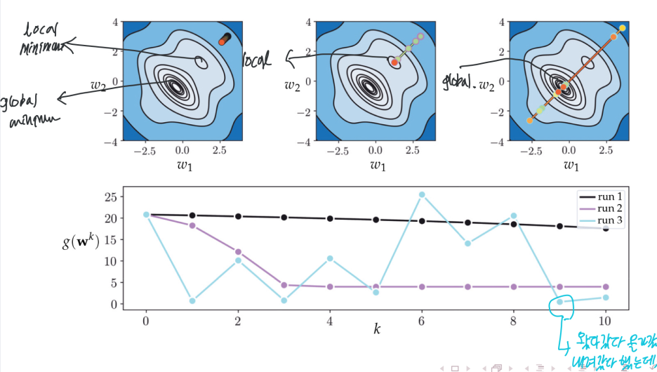
(2) 언제 멈출까? Convergence criteria

$-▽g\left(w^k\right)\sim 0_{N\times 1}$−▽g(wk)~0N×1​​

gradient가 0에 가깝다는 것은 거의 local minimum에 다가왔다는 의미가 된다. 하지만 사실 연속적인 값일 때정확히 0 값이 나올 확률은 0이다. 그래서 조금 더 자세하게 정하는 것이 필요하다.

① || ▽g(w^k-1) ||이 충분히 작을 때

② (1/N)|| ▽g(w^k-1) || < ε

② (1/N)|| g(w^k) - g(w^k-1) || < ε

 

(3) Two Natural Weakness of Gradient Descent

문제점

① Direction: rapidly oscillate during a run of gradient descent, often producion zig-zagging steps that take considerable time to reach a minimum point. (contour plot에 gradient가 수직이라 지그재그로 내려가게 되는 상황

② Magnitude: local minimum에서 급격하게 gradient가 작아져 optimization에 매우 오래 걸림

 

해결방안

① Direction(Zig-zagging): EWMA(Exponential Weighted Moving Average)

$d^{k-1}=\left(1-\beta \right)d^{k-1}-\beta ▽g\left(w^{k-1}\right)$dk−1=(1−β)dk−1−β▽g(wk−1)​

이전 진행 방향과 이번 진행 방향의 값에 가중치를 두어 oscillation을 줄이는 방법.

 

② Magnitude(Slow-crawling): normalized gradient descent

즉, gradient는 '방향'만 제공하고 크기는 고려하지 않는다.

---

이제보니 첨자 위치에 따라 의미가 달라지는데 이전 게시물에서 이를 좀 혼동해서 적었다.

윗첨자로 되어있는 건, n번째 vector라는 의미이다.

$w^n=nth\ \left\{w_0,\ w_1,...,w_k\right\}$wn=nth {w0​, w1​,...,wk​}​

반면 아래첨자로 되어있는 건, model의 n번째 parameter라는 뜻이다.

---